NMR (optional)
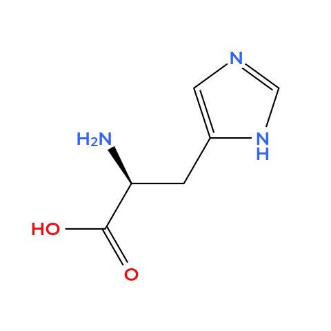
Important application of computational methods is supporting the analysis of experimental spectra. Nuclear magnetic resonance (NMR) spectroscopy is one of the most frequently used methods for structure elucidation or evaluation of reaction products in an experimental setting. Often, the molecules of interest are flexible organic molecules. Therefore, in order to reproduce experimental NMR spectra it can be paramount to use an ensemble approach for the calculation of the spectrum, because of the dependence of chemical shifts and, even more so, coupling constants on the molecular geometry. L-Histidine is a natural product that shows this behavior. Your task going forward is to calculate the NMR parameters of L-Histidine using the Conformer-Rotamer Ensebmle Sampling Tool (CREST) and Command-line Energetic Sorting of Conformer-Rotamer Ensembles (CENSO) programs to first generate an ensemble and then calculate the 1H-NMR parameters.
Ensemble Generation
To generate an initial ensemble, you are going to use a meta-dynamics approach using CREST. For this exercise CREST will be run using default settings, although we want to use an implicit solvation model in the meta-dynamics
crest l-histidine.xyz --alpb h2o > crest.out &
20
6274
O     -1.0689000000   -1.6919000000   -0.7660000000
O     -2.4946000000   -1.1223000000    0.9038000000
N      1.6797000000    0.1409000000    1.1624000000
N     -2.7494000000    1.3693000000   -0.2178000000
N      2.8201000000   -0.3365000000   -0.6825000000
C     -0.3579000000    1.3004000000    0.3217000000
C     -1.5062000000    0.6397000000   -0.4567000000
C      0.9671000000    0.6020000000    0.1195000000
C     -1.7498000000   -0.7917000000   -0.0102000000
C      1.6556000000    0.3150000000   -1.0031000000
C      2.8043000000   -0.4249000000    0.6290000000
H     -0.5942000000    1.3196000000    1.3946000000
H     -0.2433000000    2.3450000000    0.0039000000
H     -1.3124000000    0.6416000000   -1.5355000000
H      1.4441000000    0.1943000000    2.1450000000
H      1.3992000000    0.5299000000   -2.0301000000
H     -2.6419000000    2.3346000000   -0.5280000000
H     -2.9358000000    1.4198000000    0.7835000000
H      3.5655000000   -0.8810000000    1.2458000000
H     -1.2415000000   -2.6142000000   -0.4801000000
You can define the number of cores to use with the -T argument.
For the sake of reducing computation time, we only use the output of one CREST run. However, please note that CREST’s algorithm is a stochastic process and therefore not deterministic. To get the most robust exploration of the potential energy surface, you should use the output of multiple CREST runs and use clustering. For this, please refer to the documentation.
After the CREST calculation, you will find your ensemble and some additional files in your working directory. Your ensemble will be dumped in XYZ format in a file called crest_conformers.xyz.
Ensemble Refinement and Spectral Parameter Calculation
Next, you are going to refine the ensemble using DFT calculations. CREST uses GFN2-xTB as the default method, which produces ensemble rankings that are not accurate enough for NMR calculations. Therefore, it is necessary to refine the initial ensemble. You can do this using CENSO, which is supposed to automate the process of ensemble refinement and property calculation. Before starting your calculations, please configure the program paths in the provided configuration file. You can define the number of cores for CENSO with –maxcores.
censo -i crest_conformers.xyz --inprc censo2rc_histidine > censo.out &
[prescreening]
threshold = 4.0
func = pbe-d4
basis = def2-SV(P)
prog = tm
gfnv = gfn2
run = False
template = False

[screening]
threshold = 3.5
func = r2scan-3c
basis = def2-TZVP
prog = orca
sm = smd
gfnv = gfn2
run = True
implicit = True
template = False

[optimization]
optcycles = 8
maxcyc = 200
threshold = 2.0
hlow = 0.01
gradthr = 0.01
func = r2scan-3c
basis = def2-TZVP
prog = orca
sm = smd
gfnv = gfn2
optlevel = loose
run = False
macrocycles = True
crestcheck = False
template = False
constrain = False
xtb_opt = True

[refinement]
threshold = 0.95
func = wb97x-v
basis = def2-TZVP
prog = tm
sm = cosmors
gfnv = gfn2
run = False
implicit = False
template = False

[nmr]
resonance_frequency = 600.0
ss_cutoff = 8.0
prog = orca
func_j = r2scan-d4
basis_j = def2-TZVP
sm_j = smd
func_s = r2scan-d4
basis_s = def2-TZVP
sm_s = smd
gfnv = gfn2
run = True
template = False
couplings = True
fc_only = True
shieldings = True
h_active = True
c_active = False
f_active = False
si_active = False
p_active = False

[uvvis]
prog = orca
func = wb97x-d4
basis = def2-TZVP
sm = smd
gfnv = gfn2
nroots = 20
run = False
template = False

[general]
imagthr = -100.0
sthr = 0.0
scale = 1.0
temperature = 298.15
solvent = h2o
sm_rrho = alpb
multitemp = True
evaluate_rrho = True
consider_sym = True
bhess = True
rmsdbias = False
balance = True
gas-phase = False
copy_mo = True
retry_failed = True
trange = [273.15, 373.15, 5]

[paths]
orcapath = /path/to/orca/binary
xtbpath = /path/to/xtb/binary
mpshiftpath =
escfpath =
orcaversion =
CENSO will write output for all parts in text-format, as well as in json-format (.out and .json files).
You will also find ensembles in xyz-format, as well as all files generated using the run in your working directory, sorted by section.
In the printout of the program and in the 4_NMR.out file you will find the ensemble–averaged NMR parameters.
Sodium trimethylsilylpropanesulfonate (DSS) is used as the NMR standard, and the spectrum is recorded at a frequency of 600 MHz in aqueous solution.
Compare the ensemble–averaged values and the values for the lowest conformer only to the provided experimental reference values below.
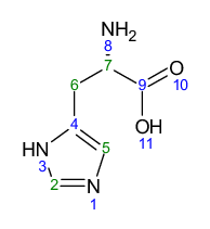
| δ (ppm) | Integral | Multiplet type | J (Hz) | Atom No. |
|---|---|---|---|---|
| 3.16 | 1 | dd | 15.55, 7.7 | 6 |
| 3.23 | 1 | dd | 16.10, 4.9 | 6 |
| 3.98 | 1 | dd | 7.73, 4.98 | 7 |
| 7.09 | 1 | d | 0.58 | 5 |
| 7.9 | 1 | d | 1.13 | 2 |